I am trying to work out where I am at....

This is a programming and project management problem.
I haven't done much programming for a while.
I am using the two blogs separately even though they are sort of combined.
Then I am using and learning R and Javascript at the same time.

It's all a bit complex!

In order to not lose my mojo, I need to work out where I am at and build in the plan to review that.


Last two edited files on my Aptana workspace was:
NFkB_Pathway_info.txt
MultipleUniprotAccNumber_Clean_20140509.html

Last git commit was on the 6th of May.

So that suggests that I haven't done any programming for 11 days...

Let's open that file and see how I do...

How the proteins array is organised...

I have created the file with the name of:
MultipleUniprotAccNumber_rearrange_array_20140520.html

Key commands for making the array

in a loop that goes through each of the IDs
   get the info from the XML file
   in loop that goes through each of the features
       protein[i] =Array(type[i], desc[i], stat[i], start[i], end[i]);
 
   then combine this with

proteins.push(protein);

Now proteins is organised with 

• an array for each protein 
• an array for each feature
• five bits of info for each feature (type, desc, status, start, end)

proteins.length give the number of proteins (ordered by UniID)

protein[i].length gives the number of features for protein[i]

proteins[2][0][0] returns the type of the first feature of the third protein. 

Now I should be able to loop through these all relatively easily. 

Today has been spent trying to learn about arrays...

I wrote the script below to try to understand how the Array function and the push function to assemble different arrays. 

<script>

  var array1 = [1,2,3,4,5];

  var alphaarray = ["a","b","c","d","e"];

  var arrayarray = [];

  var pusharray = [];

  var anotherpusharray = [];  

    

    

    for (i = 0; i < array1.length; ++i)

            {   

                arrayarray[i] =Array(array1[i], alphaarray[i]);

                pusharray.push(array1[i],alphaarray[i]);

                

            }

    

    anotherpusharray.push(array1, alphaarray)

  

     document.write("<br>");     

     document.write("<br>");

     document.write(arrayarray);

     document.write("<br>");     

     document.write("<br>");

     document.write(arrayarray[0]);

     // output put is 1,a

     

     

     document.write("<br>");     

     document.write("<br>");

     document.write(pusharray);

     

     document.write("<br>");     

     document.write("<br>");

     document.write(pusharray[0]);

     

  

  // output looks the same for both arrayarray and pusharray even though the information is differently organised.  

  // the different organisation is demonstrated by what happens when you write the first element from each array. The first element from 

  // arrayarray is [1,a]

  

   

  

      document.write("<br>");     

     document.write("<br>");

     document.write(anotherpusharray);

     document.write("<br>");     

     document.write("<br>");

     document.write(anotherpusharray[0]);

     document.write("<br>");     

     document.write("<br>");

     document.write(anotherpusharray[0][0]);

      

 // 

  

    

    </script>

Learning more about R

Some advice about R-studio from Stuar51XT through a Youtube video (https://www.youtube.com/watch?v=qHfSTRNg6jE)

some notes:
clear console: Contol L

clear workspace: clear all tab

To use a piece of script:
   Open script window
   Write script
   Highlight script
   Press run


To use a file
    Put script in a file with a .R suffix.
    source function will run the file - as long as it can find it....
    source("z.R")

Get working directory
    getwd()

Multiple panels in R

Some useful tips here:
http://www.statmethods.net/advgraphs/layout.html

Heatmaps 2

Interesting piece on the web here:
http://mannheimiagoesprogramming.blogspot.co.uk/2012/06/drawing-heatmaps-in-r-with-heatmap2.html

Data Analysis for Suliman...

So I am going to try to do this now.
I will prepare a Powerpoint file with the pictures in there and send it to Ian and Suliman for comment.

Starting about 14:15.


Cleaning the combined data frame for a heat map:
useful command is subset
> keep <- subset(cleanboth, select = -Pat_12)
This removes the data from Patient 12

> keep <- subset(keep, select = Accession)
Just leaves the Accession column...

> x <-keep[complete.cases(keep), ]
Focusses on just the samples with no missing values.
Sadly on 189 observation.

Now 15:54.

Managed to do lots of stuff but didn't manage to produce heatmap.
It thinks the data.frame is NOT numeric so it won't allow me to make the heatmap.

Try again later.

A few pages of data to send to Suliman for some feedback.

Comparing distance matrices....

So there is a test. It seems it's called the Mantel test.
More info here:
http://www.ats.ucla.edu/stat/r/faq/mantel_test.htm
and here:
http://qiime.org/tutorials/distance_matrix_comparison.html

time for some food!

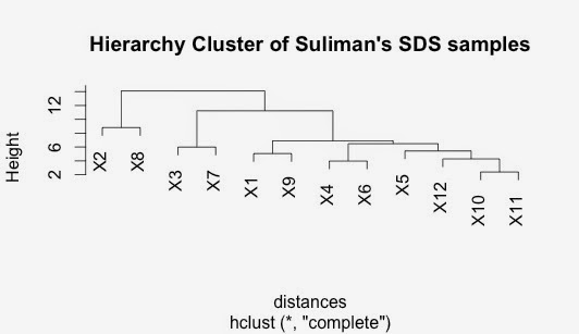
Repeat cluster analysis with SDS data...

I am repeating what I did yesterday but with the SDS data.
It seems appropriate to do these separately in the first instance.
The workflow is exactly the same but I am doing it at home on a different computer.

>summary(distances)
   Min.  1st Qu.  Median  Mean   3rd Qu.  Max. 
  2.386   5.653   6.844   7.527   9.275  14.110 

This looks similar to the range of values yesterday. 

Biggest difference: Pat 2 and Pat 3. 

Smallest difference: Pat 10 and Patient 11.

Do hierarchial cluster on this distance matrix

The SDS and the NP40 clusters has some similarities but some differences too. 

I don't really know which to focus on at the moment. 

I will have to do a little bit more work on this. 

Interestingly, the closest sample in both the NP40 data and the SDS data was Patient 10 and Patient 11. Both have very significant correlations. 

I think I need to find a way to compare two distance matricies. 

However, I am going to try to generate a heat map first. Peter Morgan advised this as a possible option. 

I am reading "Visualise This" again as there was a chapter about heatmaps there - starts on page 228. 

It is necessary to convert the data into matrix format. 

> SDS_matrix <- data.matrix(SDS)

Data is not ordered so this is likely to cause a problem, I think. 

Also there are quite a lot of missing values - again likely to cause a problem. 

I removed this samples that had any missing data (using Excel). There is a way to do this in R but I got confused. 

Then I turned it into a matrix and used the default heatmap options. These include doing a distance measure and clustering. This is the result:

The output is kind of interesting but it seems that most of the proteins do nothing. 

It might be worth doing this with the combined NP40 and SDS dataset. This would at least be larger than just the SDS dataset. 

Midday now. 

I am getting a little distracted and wandering a bit. 

I wanted to draw a boxplot of my data. 

However this generates this:

This is not very useful!!!

I need to generate the boxplot without the first column of data. 

Sadly I don't know how to do that. 

A web search found a very nice site for adding detail to boxplots:

http://www.r-bloggers.com/box-plot-with-r-tutorial/

but it didn't tell me how to remove that first column. 

Mmm, well this command works:

> boxplot(X1, X2, X3, X4, X5, X6, X7, X8, X9, X10, X11, X12)

This gives:

Again, interesting data. 

I can make this look a little better by adding labs to X-axis, correcting the spelling error in the title and putting the X and Y labs in bold. 

Here it is:

The code for this is:

> boxplot(X1, X2, X3, X4, X5, X6, X7, X8, X9, X10, X11, X12, main="SDS Data plotted by Patient Sample Number", xlab=expression(bold("Patient Samples 1 to 12")), ylab = expression(bold("Relative Quant")), las = 2, names = c("Pat 1","Pat 2","Pat 3","Pat 4","Pat 5","Pat 6","Pat 7","Pat 8","Pat 9","Pat 10","Pat 11","Pat 12"))

Breaking this down a bit:

> boxplot(X1, X2, X3, X4, X5, X6, X7, X8, X9, X10, X11, X12, 

+ main="SDS Data plotted by Patient Sample Number", 

+ xlab=expression(bold("Patient Samples 1 to 12")), 

+ ylab = expression(bold("Relative Quant")), 

+ las = 2, 

+ names = c("Pat 1","Pat 2","Pat 3","Pat 4","Pat 5","Pat 6","Pat 7","Pat 8","Pat 9","Pat 10","Pat 11","Pat 12")

+)

Remember the data was attached which means that I could use the titles. 

Good to learn this stuff. 

Enough for now. 

Playing with Suliman's proteomic data.....

I have decided to start simply in R.
I have opened a new project. This clears all the data from the memory which looks like a clean start.

Steps:

1. Get the data in..  NP40 = read.csv("...")
1. First time I did this, I used read.txt and the data was in the wrong format!
2. Look at the data.. head (NP40)
3. Attach(NP40) - then I can use the headings. This is faster than using $ all the time. 
4. Play a bit - plot(Pat_1~Pat_2)
5. Try default distance measures dist(rbind(Pat_1, Pat_2, Pat_3....)
6. rbind combines the data by rows and is required for the dist function
7. Put these in a matrix themselves distances <- dist(rbind(Pat_1, Pat_2....)
8. Do hierarchy clustering hc <- hclust(distances) and then plot(hc)

So this all worked and made a cluster and gave some distances. 

Distances:

           Pat_1     Pat_2     Pat_3     Pat_4     Pat_5     Pat_6     Pat_7     Pat_8     Pat_9    Pat_10

Pat_2   7.537715                                                                                          

Pat_3   3.875914  6.809347                                                                                

Pat_4   5.263328  8.908621  4.036732                                                                      

Pat_5   6.415988  7.497405  5.970487  6.052602                                                            

Pat_6   5.335291  7.945542  5.344391  5.737485  5.301845                                                  

Pat_7   9.638823 11.860930  8.369786  8.654071 12.813030 13.373229                                        

Pat_8  10.546800  7.906824 10.610556 11.005512 10.942666 11.187895 12.030716                              

Pat_9   5.540512  6.480492  5.825622  7.233939  5.790468  4.195550 10.479076  9.158402                    

Pat_10  4.815430  8.433853  5.014136  7.109553  5.986761  4.804471 12.413832 11.686438  5.207372          

Pat_11  4.632951  8.585297  5.024850  6.874530  5.928018  4.487083 12.188807 11.433096  4.944108  2.930767

The distances vary from 2.93 Patient 10 vs Patient 11 to 13.4 Patient 6 vs Patient 7.

> summary(distances)

   Min. 1st Qu.  Median    Mean 3rd Qu.    Max. 

  2.931   5.319   6.875   7.603  10.060  13.370 

If we plot these two it generates interesting plots:

Plot of closest Patient samples (Pat_10 vs Pat_11)

r-squared = 0.49, p<0.0001

 Plot of farthest patient samples (Pat_6 vs Pat_7)

r-squared = -0.002. p=0.43

I decided to plot the residuals of this to see if there are outliers in the data set. 

>largedist.res = resid(largedist)

This function resid calculates the residuals

> plot(largedist.res)

gives...

I think anything with a residual above 0.5 is probably interesting and may merit some investigation. Certainly, the two dots above 1.0 merit a look....

I wanted to compare a third set of data that used different patients samples but still had a large distance. I chose to

>plot(Pat4~Pat8)

which gave: 

r-squared=0.15, p>0.001

This is interesting as event though the distance is relatively large and the r-squared is quite small, the correlation is significant. 

Residual graph is here:

There maybe some interesting proteins here. 

Sadly, it is not immediately easy to work out which protein is which as we lose the protein IDs during the process. The plots don't require this. 

Interesting afternoon with lots to think about. 

Some nice productive playing with R. 

Some more questions come to mind:

• Will the SDS data generate the same hierarchy cluster as the NP40 data?
• Is there a way to evaluate distance? Do the values mean anything? I guess you can average this and then divide by the average. This might give some sort of outlier information...

That's enough for today. 

Hierarchial clustering...

For Suliman's manuscript, we have been asked to do some more statistical analysis. The reviewer particularly recommended hierarchial clustering.

Thinking about it and learning a little bit more about what is involved suggests some possible questions:

• Can we cluster our patients based on proteomic data?
• What proteins determine the hierarchies?

Some issues about normalisation come to mind. 

An interesting PDF is located at www.microarrays.ca/services/hierarchical_clustering.pdf‎. This said that "the idea of this method is to build a hierarchy of clusters, showing relations between the individual members and merging clusters of data based on similarity."

A key concept is a "distance metric" which is a measure of similarity. There are different measures of correlation. Two common ones are the Euclidean and the Pearson correlations. Euclidean distance looks at just the numbers while the Pearson correlation looks more at trends. This can give very different patterns. 

Other measures of distance include: maximum, Manhattan, Canberra, binary and Minkowski. 

"For more gene expression experiments you will likely find Pearson correlations to be more appropriate."

This website here talks about using R for hierarchial clustering. 

It talks about various linkage methods: single, median, average, centroid, Ward's, McQuitty's. 

Euclidian Distance:- Square root of sum of squares of attribute differences. 

This is going to be a learning curve!!!

Making arrays in different ways....

In order to extract data for multiple proteins, there is a requirement to work with data from multiple proteins.
The question is how to arrange this data.
This is not an trivial question.

When I was extracting the Feature data for one protein, I extracted:

• type[i]
• desc[i]
• stat[i]
• start[i]
• end[i]

in separate arrays and then I used the "array" function to stitch these all together. This worked well because it held each feature in a separate array and then held the feature list together as well. 

I could delete a row when I wanted to remove a whole feature.

However, when I tried to do this for multiple proteins, I used the "push" function. Added the information as individual pieces. Now, when I try to delete, it doesn't remove a row but rather just the individual items. 

So "push" and "array" are very different.