Turning negative values to zero....

I am working with Jo Welton to explore her proteomics data.
Our first step is to turn the negative values from her data into zeros. The negative values are there because she has subtracted backgrounds.

As ever, StackOverflow is our friend. I found this link:
http://stackoverflow.com/questions/11275187/r-replacing-negative-values-by-zero

Steps we followed:

1. Convert the column of our data frame into a vector
2. Go through the vector, find the values less than zero and make them zero
3. Convert our vector back to a data frame. 
4. Bind our data frames together. 

Here is the code:

> mUr.zero <- (dataframe$col) #makes the vector

> mUr.zero[mUr.zero <0] <- 0 # loops through the vector, finds values less than zero and replaces them with zero. 

> mUr.zero <- as.data.frame(mUr.zero) # converts into a data frame

> newdataframe <- cbind(dataframe, mUr.zero) # binds this into the data frame

Happy days - this seems to work :-)

Drawing 2D plots from FCS data in R with Bioconductor, base graphics and ggplot2

So I have spend the last few days working out how to generate nice 2D plots using flow cytometry data.

It's been interesting.

Here is the code and some nice output.


#load flowCore which allows the import of FCS files. 
source("http://bioconductor.org/biocLite.R")
biocLite("flowCore")
library(flowCore)

# import the data 
ntl<-read.FCS("A01 NTL.fcs", alter.names = TRUE)
n <- exprs(ntl)  # converts the data into a matrix
cd40L<-read.FCS("A02 CD40L.fcs", alter.names = TRUE)
c <- exprs(cd40L) # converts the data into a matrix

#BASE GRAPHICS
# Use base graphics of R to display FSC/SSC dot plots. 

par(mfrow=c(1,2)) #allows to plots to be placed side to side

plot(n[,1], n[,2], 
     pch = ".", 
     ylim=c(0,1000000),
     xlim=c(0,10000000),
     xlab="FSC-A",
     ylab="SSC-A",
     main="NTL") # this works

plot(c[,1], c[,2], 
     pch = ".", 
     ylim=c(0,1000000),
     xlim=c(0,10000000),
     xlab="FSC-A",
     ylab="SSC-A",
     main="CD40L") # this works

This is the plot produced:

#GGPLOT2
#Can also use ggplot2 to draw dot plots
library(ggplot2)

#seems ggplot only likes data frames
ndf <- as.data.frame(n) 
cdf <- as.data.frame(c)

#make the plotting objects using ggplot 
p1<- ggplot(ndf, aes(x=FSC.A, y=SSC.A)) + 
  geom_point(shape=".", colour="red") + 
  ylim(0, 500000) + xlim(0,5000000) +
  ggtitle("Samp 001, NTL & IL4")

p2<- ggplot(cdf, aes(x=FSC.A, y=SSC.A)) + 
  geom_point(shape=".", colour="red") + 
  ylim(0, 500000) + xlim(0,5000000) +
  ggtitle("Samp 001, CD40L & IL4")

multiplot(p1,p2, cols=2)

This is the output 

# 2D density plots
#with contour lines
p1 <- ggplot(ndf, aes(x=FSC.A, y=SSC.A)) + 
  geom_point(shape=".", colour="red") + 
  ylim(0, 500000) + xlim(0,5000000) +
  ggtitle("Samp 001, NTL & IL4") + 
  geom_density2d(colour="black", bins=5)

p2 <- ggplot(cdf, aes(x=FSC.A, y=SSC.A)) + 
  geom_point(shape=".", colour="red") + 
  ylim(0, 500000) + xlim(0,5000000) +
  ggtitle("Samp 001, NTL & IL4") + 
  geom_density2d(colour="black", bins=5)

multiplot(p1,p2, cols=2)

#with colour indicating density
ggplot(ndf, aes(x=FSC.A, y=SSC.A)) + 
  geom_point(shape=".", colour="red") + 
  ylim(0, 500000) + xlim(0,5000000) +
  ggtitle("Samp 001, NTL & IL4") + 
  stat_density2d(aes(alpha=..density..), geom="raster", contour = FALSE)

Some very useful help from here:
http://www.talkstats.com/showthread.php/52675-ggplot2-contour-chart-plotting-concentrations/page2

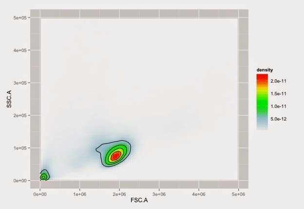
#with more colours indicating density
colfunc <- colorRampPalette(c("white", "lightblue", "green", "yellow", "red"))
ggplot(ndf, aes(x=FSC.A, y=SSC.A)) +
  ylim(0, 500000) + xlim(0,5000000) +
  stat_density2d(geom="tile", aes(fill = ..density..), contour = FALSE) +
  scale_fill_gradientn(colours=colfunc(400)) + 
  geom_density2d(colour="black", bins=5)

Cells on NTL with nice colours

ggplot(cdf, aes(x=FSC.A, y=SSC.A)) +
  ylim(0, 500000) + xlim(0,5000000) +
  stat_density2d(geom="tile", aes(fill = ..density..), contour = FALSE) +
  scale_fill_gradientn(colours=colfunc(400)) + 
  geom_density2d(colour="black", bins=5)

Cells on CD40L with nice colours

#function to allow more than one ggplot on a page
multiplot <- function(..., plotlist=NULL, file, cols=1, layout=NULL) {
  library(grid)
  
  # Make a list from the ... arguments and plotlist
  plots <- c(list(...), plotlist)
  
  numPlots = length(plots)
  
  # If layout is NULL, then use 'cols' to determine layout
  if (is.null(layout)) {
    # Make the panel
    # ncol: Number of columns of plots
    # nrow: Number of rows needed, calculated from # of cols
    layout <- matrix(seq(1, cols * ceiling(numPlots/cols)),
                     ncol = cols, nrow = ceiling(numPlots/cols))
  }
  
  if (numPlots==1) {
    print(plots[[1]])
    
  } else {
    # Set up the page
    grid.newpage()
    pushViewport(viewport(layout = grid.layout(nrow(layout), ncol(layout))))
    
    # Make each plot, in the correct location
    for (i in 1:numPlots) {
      # Get the i,j matrix positions of the regions that contain this subplot
      matchidx <- as.data.frame(which(layout == i, arr.ind = TRUE))
      
      print(plots[[i]], vp = viewport(layout.pos.row = matchidx$row,
                                      layout.pos.col = matchidx$col))
    }
  }
}

Clearing the environment in R

from here: http://www.statisticsblog.com/2010/04/r-clean-up-your-environment/

USE WITH CAUTION

rm(list = ls())

Learning how to graph flow cytometry data in R.... day one

I found this very interesting tutorial here:
http://bioinformatics.ca//files/public/Flow_2013_Module2.mp4

It goes through some of the key concepts to analyse flow cytometry data in R.

These include:

• vectors
• binding two vectors into a matrix
• lists
• mylist <- list(“first” = x, “second” = y)
• x and y are vectors that were defined earlier. 
• Thus the list here contains vectors. 
• INTERESTING AND IMPORTANT
• defining within a list uses double square brackets:
• mylist[[1]]
• can call a part of a list by it’s name!
• mylist[[“first”]]
• access by name rather than by index number can be very useful if multiple names are the same or if index numbers change.
• length(mylist)
• subsetting by index or name.
• Fundamental to R
• variables
• functions
• syntax of commands
• round brackets for functions; square brackets for subsetting
• data structures
• nest functions within functions - innermost brackets first.
• Google the error messages!
• warning messages rather than errors

Comment: I did this with Jo a little bit and made some notes but I don’t know where they are.

functions that are useful for subsetting for flow cytometry data:

• which - returns the index which adhere to the key concepts. 
• intersect
• union

Visualising flow cytometry data

• plot(density(a))

Key package - flowCore - it's a Bioconductor Package

Installing flowCore:
> source("http://bioconductor.org/biocLite.R") 

> biocLite("flowCore")

When we import an FCS file into R using read.FCS, it creates a special kind of object called a flowFrame. This seems to act like a kind of data frame with lots of metadata and the like. 

The data from this flowFrame can be converted into a matrix which can be useful. 

Another key package - flowViz

Installing flowViz:

> biocLite("flowViz")

this allows plotting of data but is quite slow!

Using "@" symbol to explore an object. 

I am having some problems with flowVis. It's giving an "Error: subset out of bounds" message. 

If I extract the data then I can plot the data nicely:

E <- exprs(data)

plot(E[,1], E[,2], 

     pch = ".", 

     ylim=c(0,1000000), 

     xlab="FSC-A",

     ylab="SSC-A",

     main="Forward Scatter vs Side Scatter") # this works

This gives a graph like this:

IT'S SLOW BUT IT IS PROGRESS...

with and by in R

These are important commands but not really commands that I understand in detail.

http://www.statmethods.net/stats/withby.html

Getting help....

help() OR ?
e.g. help(hist) OR ?hist

help.search() OR ??

demo()
   Not all functions have demos but some do!
e.g. demo(graphics)


vignette()
    Usually points at a PDF.

From the course on pluralsight

Basic R commands again

This link is useful:

http://www.calvin.edu/~scofield/courses/m143/materials/RcmdsFromClass.pdf